But a table full of transactional data isn’t a forecast. It’s just history. To predict the future, we need to train a machine learning model to learn from past patterns. In this post, we are going to dive into time series forecasting with OML4Py by doing three major things:
- Transform our raw data into a clear daily sales trend from thousands of individual sales records.
- Execute a Pandas train-test split in Oracle SQL to evaluate our model’s accuracy on unseen data.
- Train a Prophet model in the Oracle database and securely save the resulting model to the OML Datastore.
If you are new to this, don’t worry. We’ll try to break down every single piece of logic in the simplest way possible.
Step 1: Aggregate Daily Sales and Create a Train/Test Split
Before training any machine learning model, the data needs to be shaped. Our current table (ONLINE_RETAIL) lists individual purchases. But the Prophet forecasting library doesn’t care about who bought what at 10:03 AM. It cares about how much was sold in total on that day. For time series, this means two crucial things
- Time Series Format: We must aggregate daily sales and rename the columns to the Prophet library standard: ds (for date) and y (for value).
- Train/Test Split: We designate the last 30 days of data as the “Test Set”. The rest becomes the “Train Set”
Defining the Python Scripts with sys.pyqScriptCreate
We define two separate Python functions using sys.pyqScriptCreate. Both scripts load the same raw data, but the final filtering logic sets them apart. The get_train_data script calculates the SalesTotal (Quantity * UnitPrice), aggregates it by date, finds the cutoff date (the last 30 days), and then filters to keep everything BEFORE the cutoff
Script A: Getting the Training Data
BEGIN
sys.pyqScriptCreate(‘get_train_data’,
‘def get_train_data(df_final):
import pandas as pd
# 1. Calculate Total Sales per transaction
# We multiply Quantity by UnitPrice to get the total cash value
df_final[“SalesTotal”] = df_final[“Quantity”] * df_final[“UnitPrice”]
# 2. Group by Date
# We squash all transactions from one day into a single number
daily_sales = df_final.groupby(df_final[“InvoiceDate”].dt.date)[“SalesTotal”].sum().reset_index()
# 3. Rename columns for Prophet
# Prophet assumes the date column is “ds” and the value is “y”
daily_sales.columns = [“ds”, “y”]
daily_sales[“ds”] = pd.to_datetime(daily_sales[“ds”])
# 4. The “Cutoff” Logic
# We decide that the last 30 days are for testing.
test_period_days = 30
cutoff_date = daily_sales[“ds”].max() – pd.Timedelta(days=test_period_days)
# 5. Filter: Keep only dates BEFORE the cutoff
train_df = daily_sales[daily_sales[“ds”] < cutoff_date]
return train_df’,
FALSE, TRUE);
END;
/
Script B: Getting the Test Data
The (get_test_data) script is nearly identical, but the final filter is reversed—it keeps only the data ON or AFTER the cutoff date. This is the data the model will predict against later
BEGIN
sys.pyqScriptCreate(‘get_test_data’,
‘def get_test_data(df_final):
import pandas as pd
# 1. Calculate SalesTotal (Using all-caps column names)
df_final[“SalesTotal”] = df_final[“Quantity”] * df_final[“UnitPrice”]
# 2. Aggregate Data to Daily Sales
daily_sales = df_final.groupby(df_final[“InvoiceDate”].dt.date)[“SalesTotal”].sum().reset_index()
daily_sales.columns = [“ds”, “y”]
daily_sales[“ds”] = pd.to_datetime(daily_sales[“ds”])
# 3. Define the Cutoff Date
test_period_days = 30
cutoff_date = daily_sales[“ds”].max() – pd.Timedelta(days=test_period_days)
# 4. Filter for the Testing Set
test_df = daily_sales[daily_sales[“ds”] >= cutoff_date]
return test_df’,
FALSE, TRUE);
END;
/
Executing pyqTableEval to Save the Split Tables in Oracle
Now we execute those scripts. Unlike Part 1 where we used pyqEval (which creates data from scratch), here we use pyqTableEval. it is used when you want to feed an existing Oracle table (ONLINE_RETAIL) into your Python script as a DataFrame.
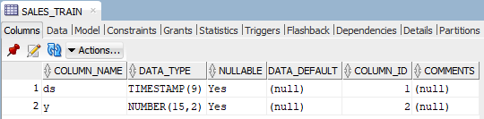
— Create the Training Table
CREATE TABLE SALES_TRAIN AS
(SELECT * FROM pyqTableEval(
‘ONLINE_RETAIL’, — The Input Table
NULL,
‘{“ds”:”TIMESTAMP”, “y”:”NUMBER(15, 2)”}’, — The Output Format
‘get_train_data’ — The Script Name
));
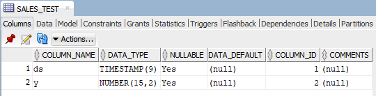
— Create the Testing Table
CREATE TABLE SALES_TEST AS
(SELECT * FROM pyqTableEval(
‘ONLINE_RETAIL’,
NULL,
‘{“ds”:”TIMESTAMP”, “y”:”NUMBER(15, 2)”}’,
‘get_test_data’
));
Step 2: Train the Prophet Model in Oracle Database
With our clean SALES_TRAIN table ready, we are now ready for the core ML process which is training the model and making sure we save the result. We are going to feed the data in SALES_TRAIN table into the Prophet algorithm.
When you train a model, you are creating a complex mathematical object. If you don’t save it, it disappears when the script ends. OML4Py allows us to save this object into a “Datastore”—think of it like a secure digital locker inside the database.
The script, train_prophet_sales, takes the training data, initializes the Prophet model with seasonality parameters (yearly and weekly patterns are common for sales data), and calls the crucial .fit(dat) method to start the learning process
How to Save a Python Model in the Oracle OML Datastore
BEGIN
sys.pyqScriptCreate(‘train_prophet_sales’,
‘def fit_prophet_model(dat, modelName, datastoreName):
import oml
from prophet import Prophet
import pandas as pd
# Prophet requires lowercase columns (ds, y)
dat.columns = [col.lower() for col in dat.columns]
# 1. Initialize the Prophet Model
# We tell it to look for yearly and weekly patterns.
model = Prophet(yearly_seasonality=True, weekly_seasonality=True, daily_seasonality=False)
# 2. Fit the model (This is where the learning happens!)
model.fit(dat)
# 3. SAVE THE MODEL to the Datastore
# This is critical. We store the “model” object under the name “modelName”
oml.ds.save(objs={modelName: model}, name=datastoreName, overwrite=True)
# Return a status message so we know it finished
return pd.DataFrame({“MODEL_NAME”: [modelName], “STATUS”: [“TRAINED”]})’,
FALSE, TRUE);
END;
/
Executing the Training Script using oml_connect:1
We execute the training script by feeding it the SALES_TRAIN database table. The most important part of this execution is passing the parameter “oml_connect”:1.
You might be wondering Why oml_connect:1? By default, Python scripts runs in a sandbox. Setting this flag to 1 gives the script permission to talk to the Oracle Database’s Datastore which is essentially a secure storage area for Python objects so it can save your model inside the database .
We run this using pyqTableEval again, but look closely at the parameters we pass in the JSON string.
SELECT *
FROM table(pyqTableEval(
‘SALES_TRAIN’, — Feed it the training data
— The Parameters:
— 1. Name the model “prophet_sales_forecast_model”
— 2. Name the locker (datastore) “prophet_sales_store”
— 3. “oml_connect”:1 <- This is the key that opens the locker!
‘{“modelName”:”prophet_sales_forecast_model”, “datastoreName”:”prophet_sales_store”, “oml_connect”:1}’,
‘{“MODEL_NAME”:”VARCHAR2(50)”, “STATUS”:”VARCHAR2(10)”}’,
‘train_prophet_sales’
));
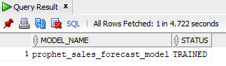
If you ran the code above and got a “STATUS: TRAINED” message, congratulations! You have officially created a machine learning model (prophet_sales_forecast_model) and saved it securely using the OML Datastore. Right now, your model is sitting natively inside the database, waiting for instructions.
By completing this tutorial, you now know how to aggregate transactional data, leverage pyqTableEval, and train a Prophet model in an Oracle database without ever exporting the data locally.
In the third and final part of this series, we will retrieve this saved model and put it to work! We’ll score the hidden SALES_TEST data to evaluate its accuracy and then generate a highly anticipated 90-day future sales forecast.
If you require any assistance regarding AI integrations, DevOps solutions, or optimizing your Oracle APEX environment, please feel free to contact us at MaxAPEX.
See you in Part 3!